City Bike Sharing

Predicting the number of bikes rented every day!

This project is aimed at predicting the number of bikes rented on a particular day using the Seoul Bike Sharing data set.

Model Development and Evaluation

A pipeline was created for data transformation and KNN regressor to prevent data leakage. Hyperparameter tuning was performed using range(2,10,2) for Discretizer Cont and Hour Transformer, Scalar Transformer Standard and MinMax, and KNN_n_neighbors = 1 was used to overfit the model to see if the data was capable of performing the prediction.

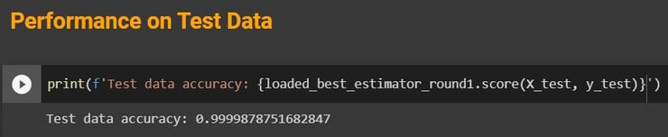
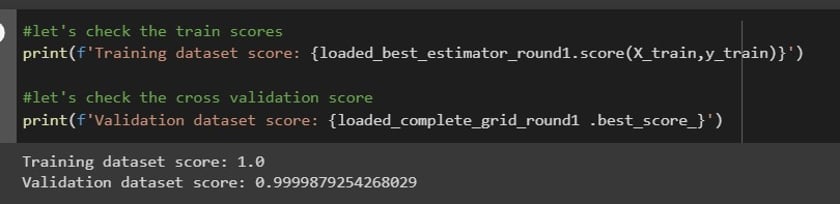
The final parameters were chosen based on validation scores, and the model was tested on test data that had not been seen by the model before. The results were a training score of 1.0, a validation score of 0.9999879, and a testing score of 0.9999878.

Conclusion

The Seoul Bike Sharing Predictive Model was able to accurately predict the number of bikes rented on a particular day. With the insights gathered from the EDA and model development, we can make better decisions regarding bike-sharing programs in Seoul.

Open in GitHub

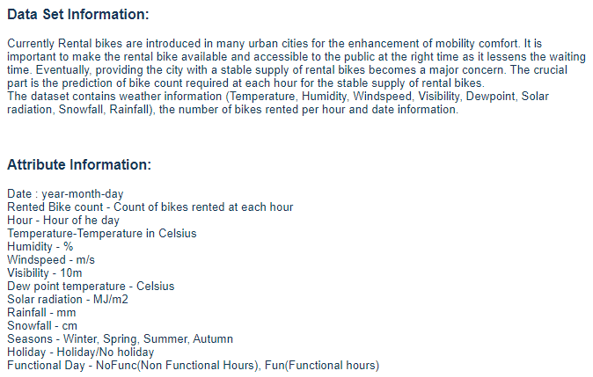
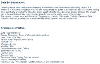
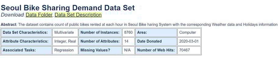
I am using Seoul Bike Sharing Demand Data Set from UCI Machine Learning Repository

Data

Procedure

Importing and Installing Packages

The main packages used were feature_ engine, sklearn, pandas, NumPy and matplotlib.

Exploratory Data Analysis

This is an essential part of each project; this is where we can get familiar with the data. I like to divide EDA into three steps.

Step 1: Look at the first few rows, familiarizing myself with the column names and their data type, checking for missing or duplicate values, and summary statistics.

Step 2: Identifying continuous, categorical, and discrete variables for further analysis.

Step 3: Visualizing the relationship between variables and correlation matrix.

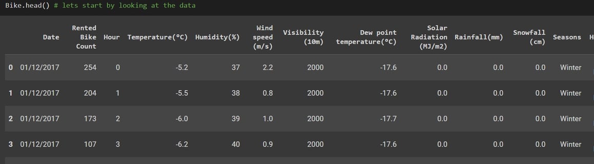
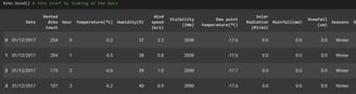
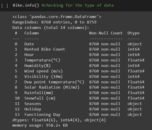
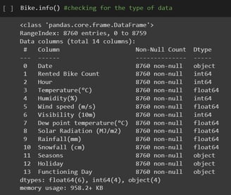
After looking at the first 5 rows of the data set, I like to call df.info() as shown in the left picture. I like this command because it gives me a lot more information other than the data type.

From this output I can see that all columns have the same number of nonnull values, so It gives me the idea that there may not be any missing values in the data, get a list of all column names and of course their data type.

Let's look at some of the EDA!

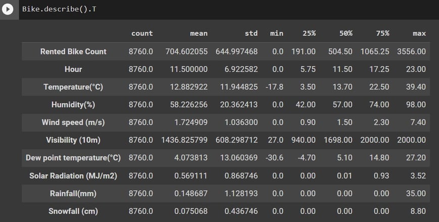
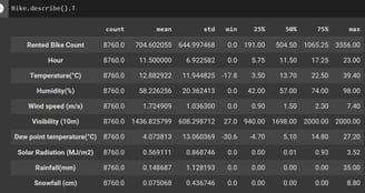
Using df.describe().T, we get a nice statistical table that is also a wealth of information.

In the table below, we are going to look at the information it is giving us, keeping in mind that this is only for numerical variables.

count: get got this from previous outputs, and we can see it is consistent through the columns.

mean: it tells us the is great variance between the variables and that I should start thinking there might be a need for variable standardization

min: shows me I have negative values in my data; this is important for variable transformation mean and median(50%): just from the difference in these values, I can see there is some skewness in the data

max: all values are greater than one, so I don't have binary variables in my data.

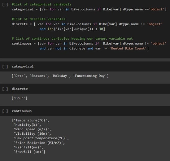
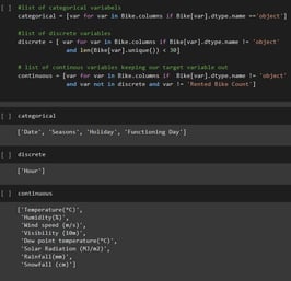
Step 2 of my process is classifying the variables into three groups, categorical, discrete, and continuous. For this classification, I have used the data type of each variable and made sure to keep the target variable out of these groups.

Step 3 is visualization of variables : In here you will see a sample of graphs used to better evaluate the data

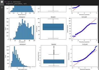
Using the continuous list of variables, I was able to obtain three graphs for each variable, as shown above. This is informative as it confirms my theory of skewness, and the box plot gives me a visual representation of outlier presence.

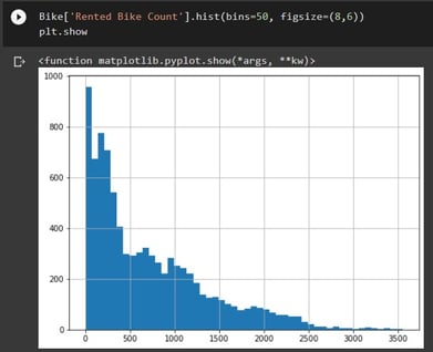
It is also important to look at the distribution of the target variable to have a true understanding of the data.

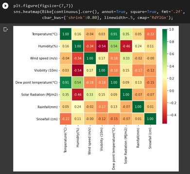
Last but not least, I like to have a correlation matrix graph. Here we can see that dew point temp and temp are highly correlated at 0.91. I want to ensure I only use one of those variables in my model.

EDA Conclusion for Pipeline Design

1. Our target variable, Rented Bike Count, is numerically continuous, so this will be a regression model.

2. There are no single-value columns.

3. We have no missing or NA values.

4. Date and functioning day are unnecessary variables. (as we are not doing a time series for this project)

5. Dew point Temp is a redundant variable that should be dropped.

6. Categorical variables need to be converted to numerical values.

7. No rare categories are present after dropping functioning day.

8. I have found significant skewness in continuous variables; since some of the variables have 0 and negative numbers we should use Yeo-Jonson transformation for Temp and wind.

9. The other continuous variables don't have a normal distribution, so we are going to discretize them.

10. There are outliers present in wind, solar radiation, rain, and snow variables.

11. We will need to do feature scaling for continuous variables to ensure all of these variables have the same scale.

Pipeline and Preprocessing Steps

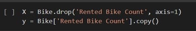
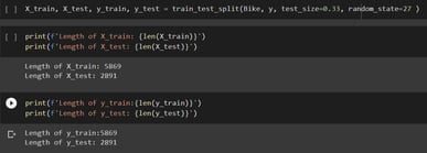
Before we do anything to the data, we want to spit it into train and test datasets.

In the pictures below, we can see that I have created two y and X variables where y is the target variable and X contains all other variables in the original data set

I have split the data in a way that the test set is one-third of the original data and the train is the remaining two-thirds.

Pipeline

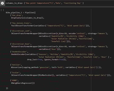
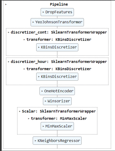
My pipeline consists of 8 steps that will happen in this specific order.

1. Drop variables Dew Point, Date, and Functioning day

2. Transform Temp and Wind Speed using Yeo_Jonson transformation

3. Discretize remaining continuous variables into 10 bins

4. discretize hour variable into 10 bins

5. One hot encode categorical and discretized variables

6. Remove outliers in temp and wind using Winsorizer

7. Scale Tmp and wind using MinMax Scaler

8. Apply KNeighborsRegressor

Hyperparameter tuning and GridSearch Coss Validation

For this project, I did three rounds of hyperparameter tuning.

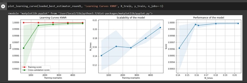
My usual approach is to try to overfit the model and to start with basic tunning in the first round. It is important to overfit the model to see if the training data has the capability to perform well with this algorithm. To overfit the model, I set the KNNR__n_neighbors to 1.

In this case, I not only obtained confirmation that the data was able to perform well, but the validation data also gave me great results. As I mentioned above, three rounds were done with similar results. I opted for using round 1 as my final model.

In the pictures below, we can see the parameter tuning step, best parameters, learning curve plots, and train and validation scores.

Testing Model Performance on Test Dataset

Let us not forget that up to now, all hyperparameters have been chosen based on the validation scores of our dataset, and the model has to be tested on a set of data that has not been seen before. That is why we have split the data from the very beginning and only worked with the training setup until now. Now we will use the model with the parameters chosen on the test set.

I am happy to report that with this model, I obtained high accuracy even in the test dataset.